Connecting R to Athena to analyse Snowplow events

We previously wrote about how to collect website data with Snowplow Analytics, save it to AWS S3, process and enrich with Lambda function and retrieve with AWS Athena.

In this post I’ll write about how to access this data through one of the most popular languages used in data science R.

AWS

Athena query result location

Assume you have your AWS Athena configured, it can query processed data. In this case you should see something like that if do a basic select query.

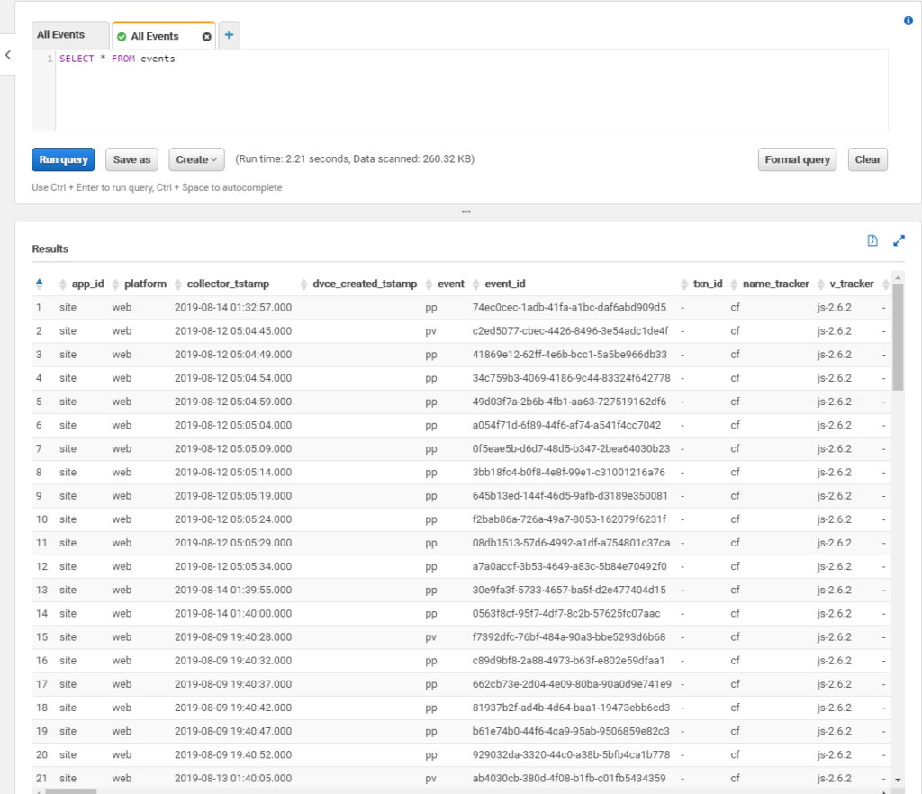
Go to Settings icon on top (not on the screenshot) and click there.

You’ll see a pop-up with Settings. Find what is in Query result location field, it should be something like s3://query-results-bucket/folder/ and copy it for future use.

AWS API user and policy

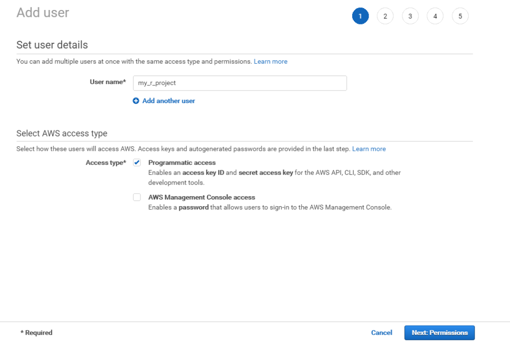
Next you need to create an API user and attach to this user an appropriate policy that allows to work with S3 and Athena. You need create user with programmatic access, because we plan to get access to Athena via API.

Then attach to this user policy, just enough to work with S3 resources where you store your data. You may find a policy that we used below:

{
  "Version": "2012-10-17",
  "Statement": [
    {
      "Effect": "Allow",
      "Action": [
        "athena:*"
      ],
      "Resource": [
        "*"
      ]
    },
    {
      "Effect": "Allow",
      "Action": [
        "glue:GetTable",
        "glue:BatchCreatePartition"
      ],
      "Resource": [
        "*"
      ]
    },
    {
      "Effect": "Allow",
      "Action": [
        "s3:PutObject"
      ],
      "Resource": [
        "arn:aws:s3:::your-bucket-name"
      ]
    },
    {
      "Effect": "Allow",
      "Action": [
        "s3:GetObject",
        "s3:ListBucket"
      ],
      "Resource": [
        "*"
      ]
    }
  ]
}

Under resource you should put your AWS bucket containing Athena files. You may use wildcard like my-bucket-* if you have multiple buckets and want to access all of them.

Finally, once the process is finished record API access key ID and secret access key, copy it somewhere for future use.

Once you have your keys, the best way to use them is to set them in your local environment. It can be done through AWS CLI (assume it is installed on your machine) with ‘aws configure” command.

You have just copied your access key ID and secret.

If you deed all things right, AWS credentials will be stored in your local environment and can be used from R. More details about the process can be found in AWS documentation.

R side

There is a wrapper package that developed by Neal Fultz and Gergely Daróczi that makes it easier to connect to AWS Athena from R. It is called AWR.Athena. You can find it on CRAN and Github.

You’ll also need DBI package to work with Athena, plus we’ll use tidyverse for data manipulation and visualisation in our example.

library(AWR.Athena)
require(DBI)
library(tidyverse)

The code below set a connection with Athena. S3OutputLocation should be taken from what you copied from your Athena settings. If you see error when trying to do that request, most probably your API user has wrong permissions.

con <- dbConnect(AWR.Athena::Athena(), region='us-west-2',
                 S3OutputLocation='s3://aws-athena-query-results-518190832416-us-west-2/',
                 Schema='default')

If all went well you can start query the database

# get list of tables available
dbListTables(con)
#query specific table  
df <- as_tibble(dbGetQuery(con, "Select * from events"))

As a result of the last command we now have all events collected in a tibble called df. I have just installed collection few days ago and the website where the tracking implemented isn’t extremely popular, so the size of resulting data isn’t an issue. If you use it in wild and with popular website, you may consider limit the data from certain date.

df1 <- as_tibble(dbGetQuery(con, "SELECT * FROM events WHERE DATE(collector_tstamp) >= DATE('2019-08-12')"))

Let’s now make a basic visualisation of the data using ggplot. What browsers did our website visitor use?

t<- df %>% group_by (br_family) %>% mutate (n=n())%>% 
        select (br_family, n) %>% count() %>% rename(browser=br_family, hits=n) %>% arrange (desc(hits))

t$browser <- as.factor(t$browser)
        

t %>%   ggplot(aes(x="", y=hits, fill=browser))+
        geom_bar(width = 1, stat="identity")+
        coord_polar(theta = "y", start = 0)

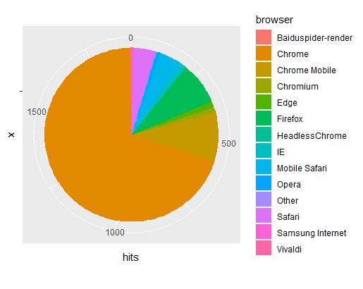
We see that the most popular browser is Google Chrome (to no surprise).

That is very simple example, just scratching the surface of what is possible to do with R. The possibilities are endless. To get full source code (with some extra examples) you can visit our Github page.